Research Journey

May 29th - June 2nd

During my first week, my teammates and I met with Chris for an explanation on the current state of the project, his expectations of us, the necessary steps to get there, scheduling for future meetings, and further explanations on how to use a beacon. A beacon is an "indoor" GPS that tracks the user's movements.

Frustrations

There was difficulty in extracting the user's movements from the manufacture's dashboard. Chris guided us in what to type in our terminal to extract the coordinates from the beacon. This took a while to figure out because Chris, my teammates and I kept getting zeros as the user's coordinates. We finally figured out we had to change some of the default configurations on the dashboard.

June 4th - June 8th

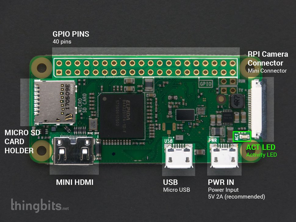
As a first time user, I focused on learning how a Raspberry Pi functions. I installed an operating system on the Raspberry Pi, and then rendered a previous group's code which created 3D audio.

Results

Rendering the 3D audio on the raspberry Pi produced a low quality wave file, which lagged frequently.

Raspberry Pi's Command Prompt

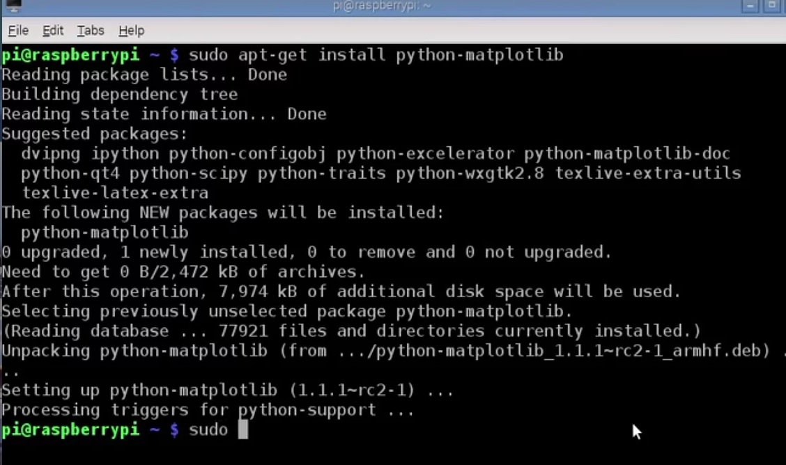
This picture shows the installation of libraries which the code we wish to run is dependent on.

Frustrations

I originally had downloaded the operating system to an old Raspberry Pi in the lab. I then had to install several libraries to get the past group's code to work. However the Raspberry Pi did not have enough memory to hold the different library downloads, thus it kept caching the libraries rather than downloading them from the website (the proper way). Professor McMullen then told me that she bought new Raspberry Pis! The libraries were then downloaded successfully (photo on the right) and I was able to render the code!

June 11th - June 15th

After getting the audio to render on the Raspberry Pi, I had to render the audio on my laptop. It wasn't as easy to run it without an IDE because my laptop runs on Windows rather than Linux or Ubuntu - an operating system optimal for computer scientists. I currently use PyCharm to run any code! My other task was to understand the fundamentals of 3D Audio. I found this part the most challenging since I have never taken a signal processing nor a 3D audio course. I delved into several topics such as head related transfer functions, head related impulse responses, interaural time difference, interaural level difference, monaural/monophonic sound reproduction, stereo sounds, convolutions, fast-Fourier transform, interpolation, sampling frequency, chunk size, time and frequency domain, and zero-padding.

3D Audio Diagram

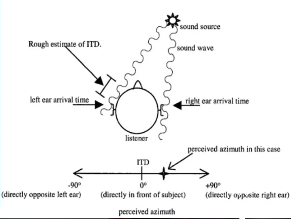
This picture shows how sound waves interacts with us given the sound source's origin.

June 18th - June 22nd

This week consisted of filling in the gaps in my understanding about the process to render 3D audio, as well as going through the work of previous groups that tried to create 3D audio. I had to identify the strength and weaknesses of the different repositories I reviewed and understand them thoroughly. The majority of them were in MATLAB, so breaking down several key concepts and understanding them well was crucial to the new implementation of the 3D audio process I would be coding in python.

Difficulties

This week was the most difficult because I wasn't sure if I understood the material well enough, but Professor McMullen helped in explaining the concepts in depth and going over each line of code for some groups.

Understanding Convolutions

A dog bark and a concert hall impulse response are convolved.

June 25th - June 30th

After understanding the fundamentals of 3D audio a well as reviewing past code repositories, the implementation process began! Out of all the data structures, I saw a hash map as the most efficient way to store the Head-Related Impulse Responses (HRIR) and Interaural Terminal Differences (ITD). Using the University California Davis's Head-Related Transfer Functions (HRTF) database, I stored subject 58's HRIR and ITD into a hash map. However, their database included HRIRs at azimuths 5 degrees apart (EX: 5,10,15..). Professor McMullen wanted the HRIRs and ITDs for one degree apart. To do this, I interpolated the data to get the extra data.Given the user's current azimuth, one can tell whether the audio enters the left or right ear first. From knowing which ear first hears the sound, I created the illusion by delaying the arrival of the sound to one of the ears. Following this, was the convolution of an HRIR with any mono sound wave; this would create the 3D audio effect. There are other necessary matrix manipulation steps to create the sound, but for simplicity, that will not be explained in this journal entry. Overall, my program would produce a sound relative to what the user should hear at a specific elevation and azimuth. The next step was to create this sound for multiple azimuths so that it appears as if sound was going in a circle around the person.

July 3rd - July 7th

After all the interpolation, convolution and matrix manipulation, I was able to get the sound. The sound looks like this: [[0, 0], [0, 0], [0, 0], ..., [0, 0], [0, 0], [0, 0]] So this week's goal was to play the sound as if it was traveling around the person's head.

Frustrations

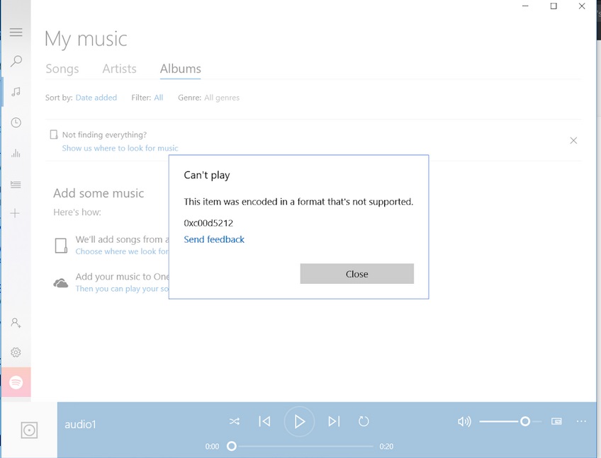
However, I was having difficulty playing the one sound I created. Luckily, Terek, one of the PhD students, helped me to get it to work. When we ran the wave file on his Mac laptop the audio played. So it was an incompatibility issue. I ended up downloading a different media player and it played the sound on my laptop.

Error Message

My First 3D Audio

This sound is at elevation 180 (behind the person) and azimuth 65. Put headphones on!

July 9th - July 13th

My next goal was to generate 3D audio in 360 degrees. At this time I didn't know how to render the audio straight from the sound card (not saving it to a wav file). The Professor wanted me to generate the 360 as a compilation of several wav files to make sure the audio sounded correctly before continuing to the next step. So I saved the sounds generated from azimuths -90 to 90 at elevation 0 and elevation 180 as wav files and combined them into one audio clip using audacity. The 360 compiled sound file sounded as it was supposed to! Now that the audio sounded correctly, I had to render the sound without exporting to a wav file.

July 16th - July 20th

I was able to render the 360 audio from the sound card (no wav file was generated), as well as manipulate how long each sound at each azimuth and elevation played. The next goal was to read this data in chunks.

Frustrations

It took me a while to read the data in chunks because several of the implementations that I tried did not work. For example, typically I could use the python method ".readframes()" however this generated the sound file in the hexadecimal format. I could not use ".readframes()" because I needed my data to be in a double or integer format. I continued looking into reading the sound in chunks

July 23rd - July 27th

This week I continued into retreiving the sound from a sound file and distorting the sound file in chunks to create the 3D audio. I still had not found a way to read the sound file in chunks so that the data retreived from it was an array of double or an integer values. I finally was able to read the sound file in chunks so that the chunk consisted of an array with double values, so that I could mathematically manipulate it (applying fourier transform and adding padding) to create the 3D audio.

July 30th - August 3rd

The previous weeks I used white noise to render the 3D audio, however now I was creating the 3D audio from the actual museum audio! This was successfully rendered without a lag on my laptop

August 6th - August 10th

My final week consisted of running the final audio sound on a Raspberry Pi. It unfortunately lagged by about 2 seconds for every change in azimuth. Finally, I had to update all my documentation and notes on github so that future groups could easily add onto the project