 Weeks 0
|
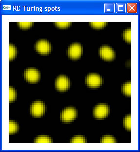
I contacted Prof. Cindy Grimm pretty early during my application to DMP 2005. After exchanging a few emails, she offered me the opportunity to come and work at Washington University as an undergraduate research intern under her guidance. Since then, through emails, she has explained to me what the project is about, and where I could find resources I needed to learn the necessary background for the project. I did my background reading well in advance and even started the first step of the project before school was over. By the time I arrived at Washington University, I had got my first tiny bit of RD code running, which is a simple implementation of Turing spot system. |
 |
Week 1 (May 30th - June 03rd)
On Monday morning, I met Prof. Cindy Grimm and Kristi Blumenberg, the other DMP intern working under Cindy's guidance this summer. It did not take much time for us to finish the administrative procedures, since Cindy had had most of this work arranged in advance. Cindy then showed us her code database and helped us set up our projects. Kristi and I were later taken out to lunch with Cindy, Prof. Bill Smart, and two other PhD students in Cindy's group - Nisha Sudarsanam and Reynold Bailey (Rennie). After that, we soon got into the regular working schedule.
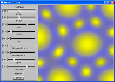
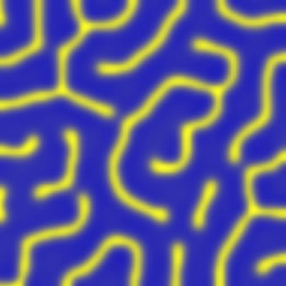
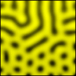
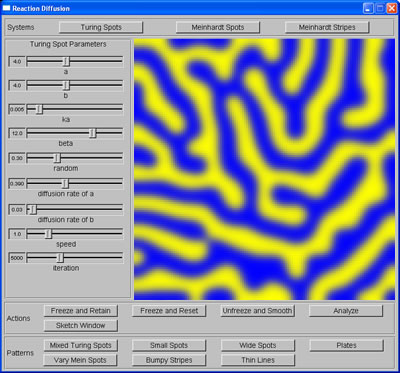
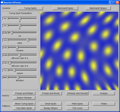
The first step is to implement Reaction-Diffusion (RD) systems basing on specifications given in Greg Turk's PhD dissertation. In his thesis, Turk described three basic RD systems: Turing spot, Meinhardt spot (also autocalystic spot), and Meinhardt stripe. As the names indicate, we can generate spots or stripes with these systems. However, when we build cascaded systems from these, we can also generate more complex patterns, such as leopard spots or mixed spots of different sizes.
On Monday afternoon, Nisha showed me how to use FLUID, a UI builder included in the open-source Fast Light Toolkit (FLTk) package, which was a big help because I needed to use this tool to build the interface for the program. By the end of the week, I had had all three basic systems running, plus two cascaded systems using Turing spot system that could produce mixed spots and leopard spots.
 Mixed spots | 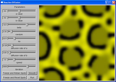 Leopard spots |
Week 2 (June 06th - June 10th)
My task for this week was to learn more about the significance of the parameters (ie. the relation between parameters of each system and the attributes of the patterns produced), as well as their ranges and their relative increments, which are important criteria for step 3: generating training data for machine learning task. To do this, I ran the program many times with different combination of parameters' values and kept notes of how the patterns changed accordingly. I spent parts of Wednesday and Thursday implementing more cascaded systems (thin stripes, mixed stripes, small spots, wide spots, and vary spots), also to learn how the attributes of the patterns can be changed further than what the parameters alone would allow.
 Mixed stripes |
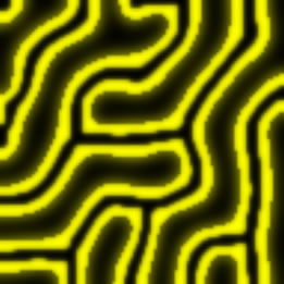
 Thin stripes |
 From stripes to spots |
On Friday, I added to my RD implementation a set of diffusion coefficients, which would pull the spots in certain directions and thus give the pattern an orientation (anisotropic patterns of spots).
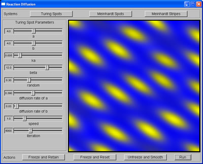
Anisotropic Turing spots
Week 3 (June 13th - June 17th)
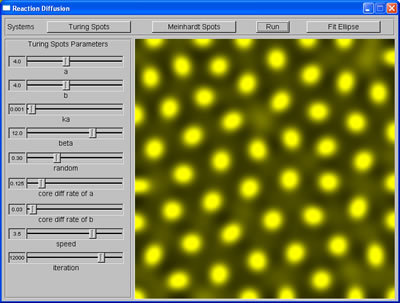
Last week I had learned a general idea about how the parameters would affect the patterns' attributes. The task for this week was to calculate numerical attributes of the patterns, such as spacing between spots, orientation and average area of the spots, etc, which was step 2 of the project. I first needed to detect the boundary of each spot so that I could fit the spots into ellipses using ellipse fitting code, which was already a part of Cindy's code database. To fit my spots into ellipses, I passed the pixels on the edge of my spots into FitEllipse function, and the function would return ellipse objects with all attributes available through member functions of Ellipse class, such as area, center's coordinates, minor/major radii and vectors. To describe a spot, I used its area to describe its size, the ratio of minor radius to major radius to describe its shape, and the major vector to describe its orientation. Then I calculated average spacing between spots by averaging the distance between each pair of adjacent spots. To do this, I used Delaunay triangulation method to decide the closest neighbors of a spot. This involved two steps:
a. Take any three ellipses at a time and use their centers to form a triangle.
b. Test every other center to see if it was inside the circumcircle of the triangle or not; if not, these three ellipses are neighbors.
 Spots produced by RD system |
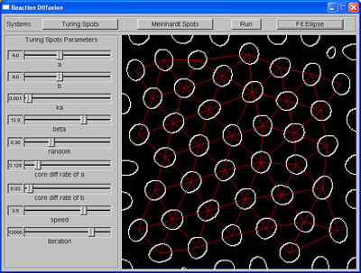 Spacings among spots are calculated |
After I had the pattern-analyzing code running, I started preparing the code to generate training data: stripping the graphics interface off, exporting the code to Linux cluster, and recompiling it under Linux. This was when I started my crash course on Linux with the tremendous helps from Robert Glaubius, the Linux man in M&M Lab, and again, Nisha (she is always willing to help!).
Week 4 (June 20th - June 24th)
The machine learning task (step 3) consists of two stages: generate thousands of lines of data by running RD systems numerous times with different parameter settings, then run machine learning code on these data so that we can map from a set of attributes to a set of correspondent parameters. To generate necessary data for the task, the RD system needed to run on a cluster of 10 Linux machines that was used for such heavy duties. This was why we needed to transfer the code to our Linux cluster and recompile it under Linux. I was mostly unfamiliar with Linux, so at first I had to rely heavily on Robert's help. After some initial problems, when Robert had finally managed to recompile the code on the cluster, we learned that the quota for my Linux account was too small to hold the program, let alone to hold the data generated. We contacted the Linux system administrator and waited for a solution.
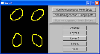
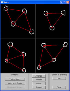
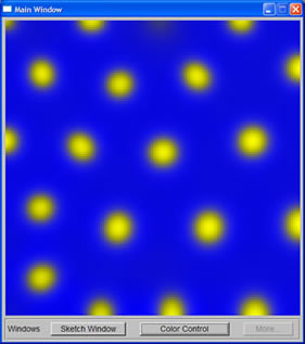
While waiting for an answer regarding the quota of my Linux account, I continued developing the program, this week, adding the sketch window, where the user can roughly sketch the pattern they want. The sketch window was divided into 4 regions to allow users to generate non-homogeneous patterns. The average area of spots sketched in each region is calculated, and then used to set up initial parameters for RD system such that the spots generated by this system will have the same size with those sketched. To test this, I wrote a simple function using linear interpolation to map from average area of spots to the correspondent value of the appropriate parameter.
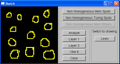 User's sketch |
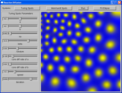 Spots produced from sketch |
Week 5 (June 27th - July 01st)
During this week, I continued working on generating data on Linux cluster, or at least tried to proceed with this task. We still had problem even after my quota has been raised up 3 times: somehow I could not create and write to files using my Linux account, and that meant I could not collect data generated by the program. We contacted the Linux system administrator again, and again waited for a solution. Meanwhile, I refined the data-generating code, adding code to detect bad textures (e.g. when the patterns are not well formed, or when the spots are too small for ellipse-fitting code). Since I changed the code, and since Robert had left for a vacation, I asked Nisha to help me with recompiling the program under Linux. We struggled for one whole afternoon, both of us not anywhere near fluent in Linux. This was when I learnt the most about compiling C code under Linux, from a simple program using one single gmake command, to a complex program using makefiles. I must say I am very much indebted to Nisha for her willingness to help.
Apart from that, I added another function to the sketch window: setting initiator cells for Meinhardt stripe system without using random factor, such that the system will generate stripes with desired orientation.
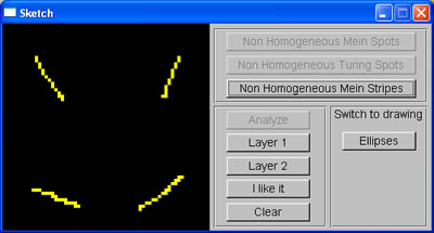 Sketch of lines |
 Stripes produced from sketch input |
Week 6 (July 05th - July 08th)
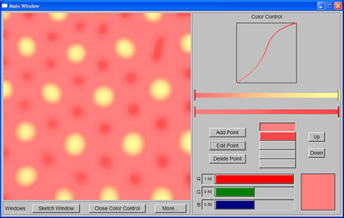
We still were not able to resolve the problem with my Linux account yet, and since I needed the result of the machine learning task to proceed with the project, Cindy asked Prof. Bill to run the program using his account instead. This was when we saw how much time it needed to run the program (hours for one data point). We then looked for ways to speed up the program, including recompiling it with faster options, and aborting execution when any chemical concentrations grew too large. Finally, the program was ready to run on Thursday, and it took only a few days to generate a little more than 15,000 data points. While waiting for the data, I worked on adding color control feature to the program, reusing the code from another program that Rennie and James Tucek (another graduate student in M&M Lab) had written a few years before.
Week 7 (July 11th - July 15th)
|
The first few days of the week were spent on completing the color control that make use of Berzier curve, and at the same time, restructuring the code of the whole program by breaking it into different classes. I spent the rest of the week on machine learning task. I rearranged the data points into four different sets (two for Turing Meinhardt spots' orientation and two for size and spacing) and then pruned them, eliminating those that were obviously erroneous. Since we were going to use Locally Weighted Regression (LWR) code written in Matlab (by Schaal & Atkeson) to do the machine learning task, I spent Thursday and Friday familiarizing myself with Matlab as well as learning how to use LWR code. |
 Week 8 (July 18th - July 22nd)
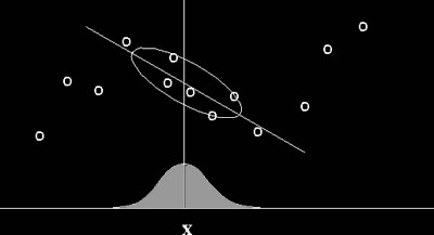 Locally Weighted Regression (image courtesy of Center for Biological and Computational Learning, Massachusetts Institute of Technology) |
Locally Weighted Regression is a memory-based algorithm for learning continuous curves that uses only training data close to the point X in question. Points nearby are weighted by their distance to point X, and then a nonlinear regression (an estimation technique using interpolation to predict one variable from one or more other variables) is calculated using these weighted points. We chose to use LWR because it does not require an extremely large collection of training data, and yet it is highly efficient for learning complex mappings from real-valued input vectors to real-valued output vectors using noisy data. The Matlab function that we used for this task was presented by Schaal and Atkeson in their paper Assessing the quality of learned local models (1994). Most of this week was spent on writing and running machine learning code in Matlab. I first ran LWR to find the optimal distance metric D, and then, using this D, I removed data points that tend to yield erroneous results. This further pruning process was done to all four sets of data points. Using a memory-based for machine learning also meant we had to store the training data and run machine learning code on them everytime we wanted to map a set of attributes to a set of parameters. Since we did not have any way to export Matlab code to C code (we needed Matlab Compiler for that), I decided to call Matlab from C code using system command to run LWR fitting, then have Matlab write the results to a text file, and finally use C code to read in the results. Of course this was not an elegant solution, but at least it did the work. |
After I had this part run as I wanted, I ran the program with different sketched patterns to test the quality of the parameters produced by machine learning mapping. Now even the orientation of the spots also differed over four regions as outlined in user's sketch. After many trials, I concluded that while the orientation mapping seemed to yield good results, the size and spacing mapping did not. I discussed this with Cindy, and we both agreed on building a linear interpolation function for size and spacing mapping, much like what I had used to test the sketching window during week 4.
 User's sketch |
 Spots produced from sketch |
Week 9 (July 25th - July 29th)
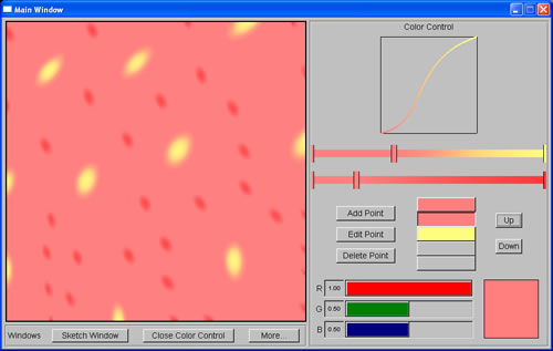
The first couple of days were spent to complete the program so that it ran as I wanted. When I showed it to Cindy, she suggested a few more improvements, including generating spots with desired spacing, and changing the color system such that spots generated by the first system can have a different color from the color of those generated by the second system. The rest of the week was spent on implementing these features.
In order to generate spots with wide spacing, I used the cascaded system susggested in Turk's paper. The first RD simulation created spots with specified spacing. The concentration of the chemicals then was used to set up the initial random factor for the second simulation, which decided where the spots would grow. The second simulation then yielded spots of desired size with the desired spacing.
 |
 Small spots with large spacing, as depicted in sketch window |
Week 10 (Aug. 01st - Aug. 05th)
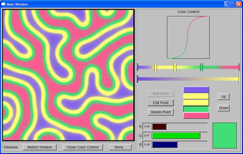
I finally finished implementing the two-color system for the program by the end of Monday. The program was more or less completed. Of course there was still more that can be done to make it better, but I decided to first build the website required by DMP. After that, I could always go back and do more work for the program.
 |
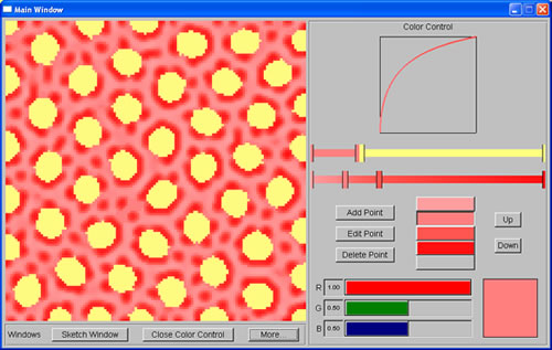 |
| Yellow spots are generated by the first system, while red spots are generated by the second system | |
I finished the rough draft of the website on Thursday, so Friday and the next Monday were spent on more work for the program. The first cosmetic improvement was the use of linear interpolation to increase the resolution of the texture produced. Then I continued working on having the system produce a pattern that had both the spacing and the orientation as sketched. Due to the way the systems worked based on the parameter settings, Turing spot system would not give me this effect, while Meinhardt spot system did. With the right level of random factor, Meinhardt spot system gave good texture. I could also freeze the first layer of spots and have the system to produce the second layer, but the outcome of this second layer depended on the spacing among the first spots and the size of the second spots. For this, more trying and testing is needed to find optimal settings.
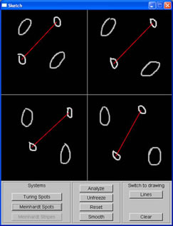 Sketching window with spots of different orientation and spacing |
 Pattern produced using Meinhardt spot system |